Approximate fit indices

Introduction

In SEM, one of the first steps is to evaluate the model’s global fit. This is commonly done by presenting multiple fit indices, with some of the most common being based on the model’s $\chi^2$ . We have developed Bayesian versions of these indices (Garnier-Villarreal and Jorgensen 2020) that can be computed with blavaan.

Noncentrality-Based Fit Indices

This group of indices compares the hypothesized model against the perfect saturated model. It specifically uses the noncentrality parameter $\hat{\lambda} = \chi^2 - df$ , with the df being adjusted by different model/data characterictics. Specific indices include Root Mean Square Error of approximation (RMSEA), McDonald’s centrality index (Mc), gamma-hat ( $\hat{\Gamma}$ ), and adjusted gamma-hat ( $\hat{\Gamma}_{adj}$ ).

We will show an example with the Holzinger and Swineford (1939) example. You first estimate your SEM/CFA model as usual

HS.model <- ' visual  =~ x1 + x2 + x3
              textual =~ x4 + x5 + x6
              speed   =~ x7 + x8 + x9 '

fit <- bcfa(HS.model, data=HolzingerSwineford1939, std.lv=TRUE)

You then need to pass the model to the blavFitIndices() function

gl_fits <- blavFitIndices(fit)

Finally, you can describe the posterior distribution for each of the indices with their summary() function. With this call, we see the 3 central tendency measures (mean median, and mode), the standard deviation, and the 90% Credible Interval

summary(gl_fits, central.tendency = c("mean","median","mode"), prob = .90)

## 
## Posterior summary statistics and highest posterior density (HPD)
##  90% credible intervals for devm-based fit indices:
## 
##                EAP Median   MAP    SD lower upper
## BRMSEA       0.099  0.098 0.097 0.005 0.090 0.107
## BGammaHat    0.956  0.957 0.958 0.005 0.949 0.963
## adjBGammaHat 0.907  0.908 0.910 0.010 0.891 0.922
## BMc          0.902  0.904 0.906 0.010 0.886 0.918

Incremental Fit Indices

Another group of fit indices compares the hypothesized model with the worst possible model, so they are called incremental indices. Such indices compare your model’s $\chi^2_H$ to the null model’s $\chi^2_0$ in different ways. Indices include the Comparative Fit Index (CFI), Tucker-Lewis Index (TLI), and Normed Fit Index (NFI).

To estimate these indices we need to define and estimate the respective null model. The standard null model used by default in frequentist SEM programs (like lavaan) includes only the indicators variances and intercepts, and no covariances between items.

You can specify your null model by including only the respective indicator variances in your model syntax, such as

HS.model_null <- '
x1 ~~ x1 
x2 ~~ x2 
x3 ~~ x3
x4 ~~ x4
x5 ~~ x5
x6 ~~ x6
x7 ~~ x7
x8 ~~ x8
x9 ~~ x9 '

fit_null <- bcfa(HS.model_null, data=HolzingerSwineford1939)

Once you have your hypothesized and null models, you pass both to the blavFitIndices function, and now it will provide both types of fit indices

gl_fits_all <- blavFitIndices(fit, baseline.model = fit_null)

summary(gl_fits_all, central.tendency = c("mean","median","mode"), prob = .90)

## 
## Posterior summary statistics and highest posterior density (HPD)
##  90% credible intervals for devm-based fit indices:
## 
##                EAP Median   MAP    SD lower upper
## BRMSEA       0.099  0.098 0.097 0.005 0.090 0.107
## BGammaHat    0.956  0.957 0.958 0.005 0.949 0.963
## adjBGammaHat 0.907  0.908 0.910 0.010 0.891 0.922
## BMc          0.902  0.904 0.906 0.010 0.886 0.918
## BCFI         0.930  0.931 0.933 0.008 0.917 0.942
## BTLI         0.883  0.884 0.888 0.013 0.862 0.903
## BNFI         0.910  0.910 0.912 0.007 0.897 0.921

The summary() method now presents the central tendency measure you asked for, standard deviation, and credible interval for the noncentrality and incremental fit indices.

Access the indices posterior distributions

You can also extract the posterior distributions for the respective indices, this way you can explore further details. For example, diagnostic plots using the bayesplot package.

dist_fits <- data.frame(gl_fits_all@indices)
head(dist_fits)

##       BRMSEA BGammaHat adjBGammaHat       BMc      BCFI      BTLI      BNFI
## 1 0.10593079 0.9499973    0.8933976 0.8883160 0.9187946 0.8644212 0.8988141
## 2 0.10014752 0.9550694    0.9042111 0.8995598 0.9274858 0.8789319 0.9071878
## 3 0.09712886 0.9576242    0.9096576 0.9052313 0.9319535 0.8863909 0.9115299
## 4 0.09818988 0.9567336    0.9077589 0.9032536 0.9308408 0.8845333 0.9105678
## 5 0.09633310 0.9582868    0.9110703 0.9067033 0.9334671 0.8889181 0.9131040
## 6 0.09211234 0.9617252    0.9184007 0.9143465 0.9386225 0.8975255 0.9178845

Once we have saved the posterior distributions, we can explore the the histogram and scatterplots between indices.

mcmc_pairs(dist_fits, pars = c("BRMSEA","BGammaHat","BCFI","BTLI"),
           diag_fun = "hist")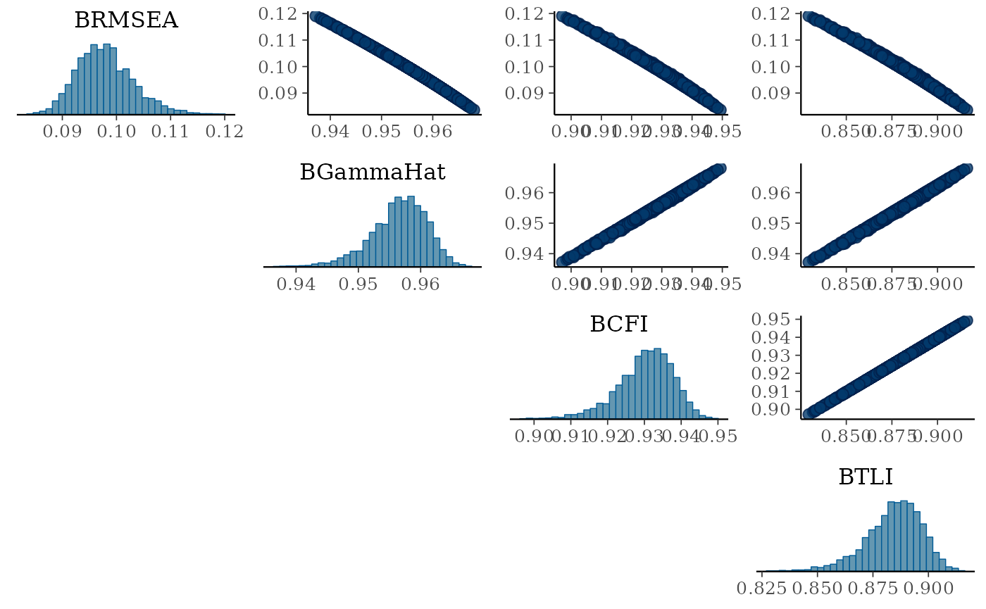

Summary

You can estimate posterior distributions for $\chi^2$ based global fit indices. Notice that here we only presented the fit indices based on the recommended method devM and with the recommended number of parameters metric loo. These can be adjusted by the user if desired.

The general recommendation is to prefer $\hat{\Gamma}$ and CFI, as these have shown to be less sensitive to model and data characteristics.

These defaults and recommendations are made based on previous simulation research. For more details about the fit indices please see Garnier-Villarreal and Jorgensen (2020).

References

Garnier-Villarreal, Mauricio, and Terrence D Jorgensen. 2020. “Adapting Fit Indices for Bayesian Structural Equation Modeling: Comparison to Maximum Likelihood.” Psychological Methods 25 (1): 46–70. https://doi.org/dx.doi.org/10.1037/met0000224.