Convergence loop

Introduction

In many cases you would need to run the BSEM models multiple times until it has converged. This can take a while and you might want to have R do it for you. This tutorial shows how to use a while loop to increase the number of burnin samples until the model converges, so you can let it run without having to adjust it every time

You will start by writing the model syntax as always. Then instead of running the blavaan functions as usual, we will run them inside the while loop as follows.

Before the loop starts you need to define a starting BURN <- 0 number of iterations, and a convergence value higher than the desired such as rhat <- 20.

Then the loop will be set stop when the convergence criteria (rhat) is lower than a desired value, like \(\hat{R} < 1.05\), we specify this with while(rhat > 1.05), meaning the the loop will continue as long as rhat is higher than 1.05.

HS.model <- ' visual  =~ x1 + x2 + x3
              textual =~ x4 + x5 + x6
              speed   =~ x7 + x8 + x9 '

BURN <- 0
rhat <- 20
while(rhat > 1.05) {
  
  BURN <- BURN + 1000 ### increase burn in by 1000 iterations every time
  
  fit <- bcfa(HS.model, std.lv=T, 
              data=HolzingerSwineford1939, 
              n.chains = 3, burnin = BURN,
              sample=1000)
  rhat <- max(blavInspect(fit, "psrf"), na.rm=T)
  print(paste0("Rhat=",rhat))  
}

Then inside the loop we will increase the number of BURN iterations by 1000 in this example. And after estimating the model, we will evaluate the convergence by getting the highest estimated \(\hat{R}\), and printing it in the screen so you will see how far is the model from converging.

print(paste0("Rhat=",rhat))

## [1] "Rhat=1.00286790201175"

Note that we are only increasing the number burnin iterations, and keeping the number of saved samples the same (1000 in this case). If you want you can increase or decrease the number of saved iterations according to your case.

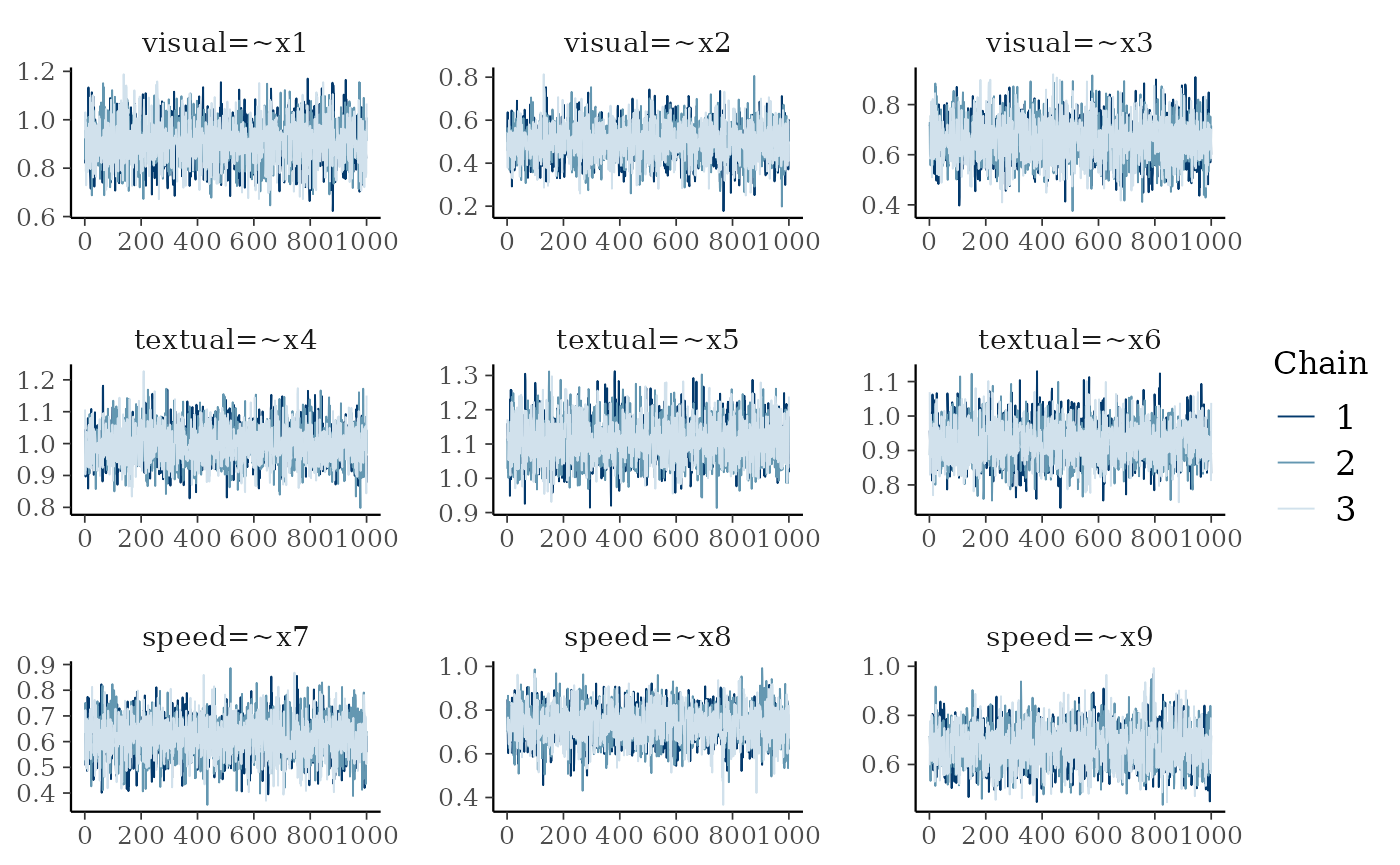
And you can visualize the convergence with the trace plots

plot(fit, pars = 1:9, plot.type = "trace")

Convergence criteria

In this example we use \(\hat{R} < 1.05\) as the convergence criteria. We recommend you to use this or \(\hat{R} < 1.01\) as the convergence criteria, but not higher.

As \(\hat{R}\) approximates 1, we can argue that the model has converged as the estimates have achieve stability between and within chains (Gelman et al. 2014)

References

Gelman, Andrew, John Carlin, Hal Stern, David Dunson, Aki Vehtari, and Donald Rubin. 2014. Bayesian Data Analysis, Third Edition (Chapman & Hall/CRC Texts in Statistical Science). Third. London: Chapman; Hall/CRC.

Convergence loop

Mauricio Garnier-Villarreal

Introduction